
The verification of sustainability claims is fundamentally shifting from broad landscape statements to precise, map-based evidence. New regulations like the EU Deforestation Regulation (EUDR) require companies to pinpoint the exact geographic coordinates of production sites, a mandate that transforms supply chain traceability.
These advancements establish a critical geospatial anchor, making it suddenly feasible to layer high-integrity biodiversity monitoring, combining remote sensing with on-the-ground bioacoustics. An integrated Nature MRV Stack moves environmental performance beyond mere declarations, showcasing verifiable changes at specific sites over defined periods.
This comprehensive overview details the essential building blocks for deploying this advanced monitoring strategy today. We explore the synergy between geofenced plot polygons, Passive Acoustic Sensors, and the analytical power of machine learning for species detection. We also address how satellite evidence helps clarify habitat disturbance context.
Crucially, the editorial outlines the limits of the technology, the necessary validation steps for ensuring honest results, and privacy-safe methods for presenting findings to regulators and stakeholders while preserving sensitive coordinates.
Key Facts: EUDR Compliance and Nature MRV Stack Components
The EU Deforestation Regulation (EUDR) is a pivotal piece of legislation requiring operators to prove that their imported products have not contributed to deforestation or forest degradation anywhere in the world after December 31, 2020. This regulation creates the primary market driver for auditable, plot-specific Nature MRV solutions, as compliance relies entirely on verifiable geographic evidence linked to the due diligence statement.
- EUDR Requires Plot Geolocation: Operators must submit geographic coordinates for production plots as part of a due diligence statement to the EU’s official information system under the EU Deforestation Regulation, with traceability and Geolocation requirements clarified in the European Commission guidance.
- Information System is Live: The EUDR Information System, built on TRACES, is the channel for submitting due diligence information, including plot coordinates, formalised by the 2024 Implementing Regulation on the EUDR Information System.
- Bioacoustics Tracks Change: Long‑term soundscape research shows acoustic community patterns can reveal degradation and recovery in tropical forests, as demonstrated by a peer‑reviewed soundscapes study in PNAS.
- Satellites Add Habitat Context: The Sentinel‑2 mission maps land cover and change, while NASA’s GEDI program provides canopy height and biomass estimates that can be clipped to the same plot polygon.
- Validation Matters: A 2024 meta‑analysis finds some acoustic indices correlate inconsistently with biodiversity in tropical biomes, which is why species‑level validation and transparent uncertainty are essential; see the landscape‑scale review of acoustic indices.
- Internal Linking Opportunity: QR-based technology can show provenance status in public views, such as through digital product passports, while precise coordinates remain in official registries.

Plot-Level Verification: EUDR Geolocation and Biodiversity Monitoring
The acronym MRV stands for Measurement, Reporting, and Verification, representing the three core pillars of credible environmental performance tracking. In the context of a Nature MRV Stack, this framework ensures that sustainability claims move beyond declarations to verifiable proof, providing the necessary transparency and data integrity for new mandates like the EUDR.
- Measurement: Collecting precise, plot-level data on biodiversity and habitat using on-site sensors, Bioacoustics, and Satellite Evidence.
- Reporting: Organising and disclosing standardised information on plot status, compliance details, and monitoring outcomes to regulators and stakeholders.
- Verification: Ensuring all data streams are auditable, scientifically robust, and validated against species-level findings and transparent error bars.
What Plot Geolocation Actually Means
Under the EU Deforestation Regulation, an operator placing in‑scope goods on the EU market must submit a due diligence statement that includes the Geolocation of the production plot. Depending on the farm size and data availability, this can be a point reference or a polygon that outlines the boundary.
Those coordinates are submitted to the Commission’s Information System through standardised fields, and they serve as the central geospatial anchor to which all other evidence can attach where required by the EU Deforestation Regulation and documented in the TRACES information system overview.
Why Coordinates Change the Evidence Standard
Biodiversity claims historically floated at the landscape level, making verification difficult. Plot geolocation fixes the unit of analysis. A buyer, an auditor, or a lender can now ask a direct question: what does the biodiversity evidence say inside this polygon for the time period that matters?
The constant nature of the polygon allows teams to combine acoustic signals from on-site sensors with satellite layers, repeating measurements to show trends instead of a single snapshot. Public comms can reference status while the sensitive geodata stays in the official system, not on a product page.
Privacy, Sensitivity, and Public View
Sensitive species and community privacy require protective measures. The safer pattern is to keep exact coordinates and raw sensor timestamps inside compliance systems, then present public‑facing summaries that state whether a plot is verified, under review, or not verified. That approach aligns with EUDR submission practice and with responsible data stewardship for Indigenous and local communities.

Data Convergence: Integrating Bioacoustics and Satellite Evidence
Bioacoustics in Plain Language
Passive acoustic monitoring uses small recorders to capture the soundscape. Machine learning can then perform two primary analytical functions. The first function is species-level detection, where trained models such as BirdNET can flag the presence of known birds with timestamps and confidence scores.
The second function involves acoustic indices that compress sound properties into numbers to track ecological change over time. Indices are cheap to compute, which makes them useful for scanning large volumes, but they are not perfect stand‑ins for species richness in every biome. A robust design pairs index‑based monitoring with a sampled subset of species‑level review so that claims rest on identifiable organisms, not only on proxies; see the landscape‑scale review of acoustic indices.
Operational Details of Passive Acoustic Monitoring
The development of a robust monitoring strategy requires deliberate trade-offs to ensure auditable data. These practical design choices directly impact the reliability and comparability of your long-term acoustic data collection:
- Recorder Density and Placement: Start with one unit per 10–25 hectares in structurally simple habitats and increase density in complex canopies. Place microphones above ground clutter where possible, or on existing infrastructure.
- Duty Cycle and Seasonality: Record at dawn and dusk when vocal activity is high, with extra coverage during migration or breeding. Keep the same schedule across months so time series remain comparable.
- QA/QC Workflow: Calibrate gain, document firmware, and retain a human‑in‑the‑loop review set. Store model versions and thresholds so results can be reproduced.
These implemented standards ensure that acoustic evidence is scientifically robust, minimising the risk of false-positive or false-negative results during compliance audits.
Satellite Layers that Add Context
Acoustics can reveal who is present and when activity changes, while Satellite Evidence gives an assessment of the habitat’s condition. Sentinel‑2 provides frequent, medium‑resolution imagery for land cover and disturbance, while Global Forest Watch utilises tree-cover loss alerts built from University of Maryland methods to provide frequent disturbance monitoring. NASA’s GEDI adds canopy height and biomass estimates from spaceborne LiDAR that can be clipped to the same polygon to interpret whether acoustic change aligns with structural habitat change.
Binding Ground and Sky to One Polygon
Export the farm boundary as GeoJSON, place acoustic points inside that boundary, and time‑stamp each file block. Clip satellite tiles to the polygon, then compute change metrics in matching windows, such as quarterly canopy height deltas or a rolling three‑month land‑cover change.
When bioacoustics and satellite signals agree, confidence rises. When they diverge, document the reason, for example, seasonal species turnover without habitat loss or canopy loss without immediate acoustic collapse.
A Demonstrated Pattern
Programmes such as Soundscapes to Landscapes show how audio and remote sensing can be fused to map species distribution and habitat relationships at scale. The same idea applies at the plot level once the polygon is known, which turns a research pattern into a compliance‑grade workflow.
Recent field reporting on remote sensing technologies and peer‑reviewed work on wildlife counting from space illustrate how remote sensing complements on‑the-ground bioacoustics when evidence is bound to the same polygon.

Implementation Guidelines for a Credible Nature MRV Deployment
Start with a 90‑Day Pilot
A short pilot validates the operational status of the stack on your plots.
In the first two weeks, draw Plot Polygons, register suppliers, and generate a sampling plan that assigns recorders to representative microhabitats. During weeks three to eight, deploy units, ingest audio to a cloud bucket, and run BirdNET on a validation subset while computing indices on the full set. Acquire Sentinel‑2 tiles and fetch GEDI products that overlap your polygons.
In weeks nine to twelve, reconcile signals, add uncertainty notes, and prepare a due diligence attachment that references your internal evidence registry without revealing coordinates in public, aligning with the EUDR Information System rules and the data conventions used by Sentinel‑2 and NASA GEDI.
Evidence Quality Rules You Can Defend
Evidence quality rules must be embedded into every step of the monitoring process to ensure the data stands up to external scrutiny. Adhering to these principles guarantees that your data is auditable, reproducible, and robust for credible claims:
- One Plot, One Truth Set: Keep a single canonical polygon per supplier lot for each reporting period, and version it when boundaries change.
- Species First, Indices Second: Use indices for efficient scanning, then justify claims with species‑level detections on a rotating validation sample.
- Transparent Error Bars: Publish the confidence logic you use, including model thresholds, false‑positive checks, and missing‑data handling for cloudy scenes.
- When to Add More Methods: In sites with heavy acoustic masking or cryptic species, add complementary evidence like eDNA water samples, which your team can introduce with a plain‑language explanation of how eDNA and satellite imagery spot subtle stress before habitat loss.
These defined standards for quality control and validation are essential elements of a defensible Nature MRV stack. They confirm that the monitoring approach is both efficient for scanning and accurate for species-level claims.
Translating Evidence into Stakeholder Disclosures
The plot results can be placed into risk, dependency, and impact categories by utilising the TNFD LEAP recommendations for metrics and targets that can be tracked over time. Teams looking ahead can position this as part of circular economy trends, which helps readers see the system-level stakes without changing the evidence standard on the ground.
Case Signals to Watch
- Degradation and Recovery: Research published in the PNAS soundscapes study demonstrates that forests broadcast their condition through the living community, allowing restoration projects to set audible goals and track progress.
- Disturbance Without Collapse: Tree‑cover loss alerts may spike without immediate species‑level declines if disturbance is patchy or seasonal, which is why both lines of evidence should be read together.
- Quiet Success: Some gains arrive as an absence of alarm rather than a loud signal. Stable canopy and steady species detections over multiple seasons are often the most credible story you can tell.

Core Analysis: Recovery, Disturbance, and Habitat Context in Bioacoustics
Recovery Signals You Can Trust
Restoration taking hold leads to a more complex soundscape. A healthy trajectory often shows rising dawn‑chorus activity across weeks, alongside an increasing share of detections from interior-forest species. It also typically reflects modest decreases in anthropogenic noise during quiet hours.
Credibility requires pairing those gains with stable or improving canopy height and biomass inside the same polygon, reducing the chance that seasonal migration alone explains the change. Keep the recorder schedule constant and report both the trend and the confidence interval so decision‑makers see progress and its uncertainty. Healthy soundscapes often track improvements in soil communities, and a deeper understanding of soil biodiversity helps teams interpret below‑ground drivers.
Disturbance and Early Warnings
Rapid drops in vocal activity in the Bioacoustics data at fixed times, sudden shifts toward generalist species, or spikes in machine or vehicle noise can indicate disturbance, and on the satellite side, short-lived fire scars, selective logging, or edge expansion may appear without total canopy loss.
Treat these as leading indicators. This should immediately trigger a field check or higher sampling frequency.
If satellite alerts appear but acoustic detections remain stable, document patchiness or the likelihood that the event occurred outside key breeding windows. As fire seasons intensify, teams must interpret short‑lived acoustic shocks alongside the growing threat of wildfires in a changing climate.
Habitat Context for Interpreting Change
Interpreting acoustic patterns becomes easier when the habitat baseline is known. Canopy height, gap fraction, and fragmentation within the polygon help distinguish genuine ecological recovery from short‑term behavioural shifts.
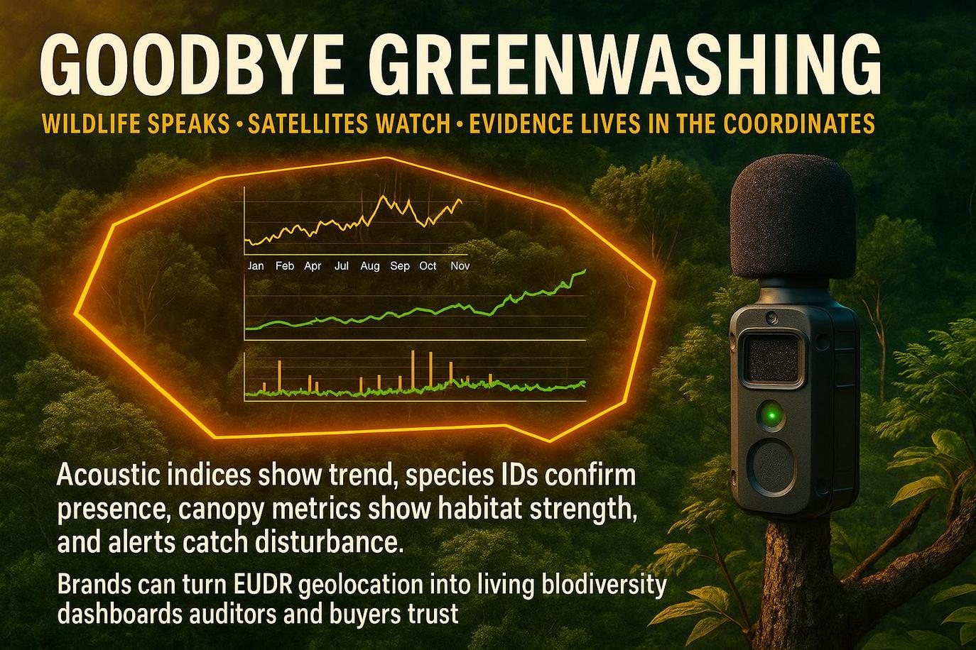
Publish a compact panel for each plot. It should show three lines: an acoustic trend, a structural habitat trend, and a simple disturbance counter.
The panel makes it harder to cherry‑pick single metrics and keeps evidence honest. The publication of the panel with reproducible code aligns field ecology with data science principles that are transforming environmental decision-making.
Deployment Insights: Quick Wins, Caveats, and Advanced Tools
Edge AI Guardians for Real‑Time Alerts
Solar audio units can flag chainsaws or vehicles between scheduled manual downloads when power and connectivity are available. Real-time alerts complement structured sampling, reducing response time for on-the-ground teams using Rainforest Connection.
eDNA as a Trigger, Not a Replacement
New methods like Environmental DNA (eDNA) can quickly reveal cryptic taxa that microphones may miss. Use it to target acoustic recorder placement and to sanity‑check index-only anomalies, especially in wetlands and riparian corridors.
Camera Traps for Focal Mammals
To observe elusive mammals, deploy a small ring of camera traps on likely paths. Camera data functions as a focal-taxon complement to the broader soundscape picture rather than a standalone verdict. Thermal imaging can extend nocturnal coverage, as demonstrated by the use of thermal scopes in conservation.
Privacy‑Safe Public Status Pages
Publish plot‑level status without sharing raw coordinates. State the monitoring cadence, last‑updated date, and whether evidence converged. Refer interested readers to your due diligence policies rather than to maps with sensitive points, and store intermediate outputs with encrypted metadata aligned to benefits of encryption for securing environmental data.
Procurement Language Vendors Can Sign
Procurement teams can define clauses that commit suppliers to polygon fidelity, minimum sampling cadence, and cooperation on incident checks. Clear expectations upstream improve the cost and time efficiency of MRV downstream. Expectations set to align with compliance-first environmental management ensure partners know the operational bar for buyers. Automation of report collation using AI-powered compliance tools reduces manual handoffs while preserving audit readiness.

Final Verification of Nature-Positive Supply Chains through Auditable Data
Adopting geofenced plots fundamentally redefines how we approach Biodiversity Monitoring, converting abstract claims into answerable questions backed by hard evidence. The true innovation lies in permanently binding high-resolution Bioacoustics and contextual Satellite Evidence to the exact same Plot Polygons. This holistic approach allows teams to conclusively demonstrate ecological recovery when it occurs, detect early disturbance signals, and present auditable, credible results to investors and regulatory bodies.
This methodology is immediately practical for any organisation navigating EUDR Compliance and provides a significant competitive edge for any buyer seeking verifiable Nature-Positive Supply Chains. The journey begins with small, deliberate pilot projects, transparently publishing your monitoring rules, and ultimately letting the data speak for itself.
As analytics mature, the applications of this modern nature MRV will increasingly intersect with future AI systems for sustainability.
Essential Questions on EUDR Compliance and Nature MRV
Is Public Disclosure of Plot Geolocation Required for EUDR Compliance?
No. Keep precise geodata inside compliance systems. Public pages can state whether a plot is verified, under review, or not verified, plus the latest update date.
Do Acoustic Indices Provide Sufficient Evidence for Biodiversity Monitoring?
No. Use indices for efficient scanning and pair them with species‑level detections on a rotating validation subset. Report error bars and threshold choices.
Key Satellite Layers for Structural Habitat Context
Begin with Sentinel‑2 for land‑cover and change products and add canopy or biomass layers that overlap your polygon. Cloud cover may require longer windows.
Determining Recorder Density for Effective Bioacoustics Sampling
Start with conservative density, then increase in complex canopies or noisy edges. A midpoint review usually pays for itself in better placement and fewer false alarms.
Establishing a Consistent Sampling Cadence for Monitoring Trends
Fix a cadence that captures seasonal dynamics, then keep it constant so trends are comparable. Increase frequency temporarily after disturbance alerts.
Elements of a Defensible and Transparent Disclosure Statement
One polygon per lot, transparent method notes, uncertainty language that matches the analysis, and an incident protocol that shows how you act when signals change.


